Ramberg Osgood material law
Introduction and governing equations
The ramberg osgood material law can be used to model
ductile behaviour for monotonic loading and is often used in fracture mechanics
applications. In contrast to
incremental plasticity models stress and strain are directly
related and thus the ramberg osgood model is in fact a nonlinear elastic model.
While algorithmically the solution of the ramberg osgood constitutive law
in a FE code is rather simple, it involves the solution of a power law (on integration
point level) which can be challenging with regard to the implementation in FEniCS (dolfin version 2019.1.0).
As in the other examples in the following we subclass the dolfin.NonlinearProblem to interact with the
dolfin.NewtonSolver and solve the linearized principle of vitual power in each iteration. The consistent
tangent and stress are functions in a quadrature space and filled manually after solving the
constitutive equations in a pure numpy code.
Linearized principle of virtual power:
Constitutive law
For the sake of brevity we skip a derivation of the equations only summarize the ones essential for the presented implementation. The strain is given by
where the stress deviator is denoted by \(\boldsymbol \sigma'\) and the equivalent stress is
\(E, \nu, \alpha, n\) and \(\sigma_{\mathrm{y}}\) are material parameters (bulk modulus \(K\) and shear modulus \(G\) are given in terms of \(E\) and \(\nu\)).
Inversion of the strain stress relation:
Equivalent stress and equivalent strain are related via a power law and for given \(\varepsilon_{\mathrm{v}}\) we can determine \(\sigma_{\mathrm{v}}\) by finding the root of:
Consistent tangent:
- Algorithm to compute stress and consistent tangent for a given strain state:
Compute equivalent strain \(\varepsilon_{\mathrm{v}}\),
Compute equivalent stress \(\sigma_{\mathrm{v}}\) via newton method (previous stress state can be used as initial guess),
Compute stress,
Compute consistent tangent
from helper import *

import matplotlib.pyplot as plt
from matplotlib.ticker import FormatStrFormatter
import numpy as np
Solution of the constitutive law
The solution of the power law mentioned above makes a vectorization of the numpy code difficult. Hence we could use a C++ function/class to solve the constitutive law. Another option is the use of numba to speed up the numpy code.
import numba

@numba.njit
def solve_ramberg_osgood(E, NU, ALPHA, NEXP, SIGY, NGAUSS, GDIM, STRAIN, STRESS):
    """solve ramberg osgood constitutive equation for each integration point in
    the computational domain

    Parameters
    ----------

    E : float
        young's modulus
    NU : float
        poisson ratio
    ALPHA : float
        ramberg osgood parameter 1
    NEXP : int
        ramberg osgood paramter 2
    SIGY : float
        yield stress
    NGAUSS : int
        total number of gauss points
    GDIM : int
        geometrical dimension
    STRAIN : np.ndarray
        strain value of each cell in Omega
    STRESS : np.ndarray
        previous stress state

    Returns
    -------
    STRESS : np.ndarray
        stress for each integration point
    DDSDDE : np.ndarray
        tangent for each integration point
    """

    LAMBDA = E * NU / (1 + NU) / (1 - 2 * NU)
    MU = E / (2 * (1 + NU))
    K = E / (1 - 2 * NU)  # bulk modulus

    DDSDDE = np.zeros((NGAUSS, GDIM * 2, GDIM * 2))

    if GDIM == 2:
        Cel = np.array(
            [
                [LAMBDA + 2 * MU, LAMBDA, LAMBDA, 0.0],
                [LAMBDA, LAMBDA + 2 * MU, LAMBDA, 0.0],
                [0.0, 0.0, 0.0, 0.0],
                [0.0, 0.0, 0.0, 2 * MU],
            ]
        )
    elif GDIM == 3:
        Cel = np.array(
            [
                [LAMBDA + 2 * MU, LAMBDA, LAMBDA, 0.0, 0.0, 0.0],
                [LAMBDA, LAMBDA + 2 * MU, LAMBDA, 0.0, 0.0, 0.0],
                [LAMBDA, LAMBDA, LAMBDA + 2 * MU, 0.0, 0.0, 0.0],
                [0.0, 0.0, 0.0, 2 * MU, 0.0, 0.0],
                [0.0, 0.0, 0.0, 0.0, 2 * MU, 0.0],
                [0.0, 0.0, 0.0, 0.0, 0.0, 2 * MU],
            ]
        )

    zero_strain_tolerance = 1e-12
    sv_tol = 1e-12
    maxiter = 50
    # helpers voigt notation
    I2 = np.zeros(GDIM * 2, dtype=np.double)  # Identity of rank 2 tensor
    I2[0] = 1.0
    I2[1] = 1.0
    I2[2] = 1.0
    I4 = np.eye(GDIM * 2, dtype=np.double)  # Identity of rank 4 tensor

    for n in range(NGAUSS):
        # strain at time t + delta t
        eps = STRAIN[n]
        tr_eps = np.sum(eps[:3])
        eps_dev = eps - tr_eps * I2 / 3
        ev = np.sqrt(2.0 / 3.0 * np.dot(eps_dev, eps_dev))

        if ev < zero_strain_tolerance:
            # return elastic tangent
            STRESS[n] = Cel @ eps
            DDSDDE[n] = Cel
        else:
            # compute correct tangent and stress
            # stress at time t
            sig = STRESS[n]
            tr_sig = np.sum(sig[:3])
            sig_dev = sig - tr_sig * I2 / 3
            # equivalent stress at time t is used as initial guess
            sv_initial = np.sqrt(3.0 / 2.0 * np.dot(sig_dev, sig_dev))

            # stress at time t + delta t
            if sv_initial <= SIGY:
                sv = sv_initial
            else:
                # initial_guess is > sigy
                sv = (SIGY ** (NEXP - 1.0) * E * ev / ALPHA) ** (1.0 / NEXP)

            def f(x):
                stuff = 1.0 / (2.0 * MU) + 3.0 / (2.0 * E) * ALPHA * (x / SIGY) ** (
                    NEXP - 1.0
                )
                return stuff * 2.0 / 3.0 * x - ev

            def df(x):
                return 1.0 / (3.0 * MU) + NEXP * ALPHA / E * (x / SIGY) ** (NEXP - 1.0)

            s = f(sv)
            ds = df(sv)

            niter = 0
            while abs(f(sv)) > sv_tol:
                sv = sv - s / ds
                s = f(sv)
                ds = df(sv)
                niter += 1
                if niter > maxiter:
                    break

            sig_dev = 2.0 * sv / 3.0 / ev * eps_dev
            tr_sig = K * tr_eps
            sig = tr_sig * I2 / 3.0 + sig_dev
            STRESS[n] = sig

            nenner = sv / (3.0 * MU) + ALPHA * NEXP * SIGY / E * ((sv / SIGY) ** (NEXP))
            tangent = 2 * sv / 3 / ev * (
                I4
                - 2.0
                / 3.0
                / ev
                * (1.0 / ev - 1.0 / nenner)
                * np.outer(eps_dev, eps_dev)
            ) + 1.0 / 3.0 * (K - 2 * sv / (3 * ev)) * np.outer(I2, I2)
            DDSDDE[n] = tangent
    return STRESS, DDSDDE
Voigt notation
It is common practice in computational mechanics to only store six of the nine components of the symmetric (cauchy) stress and strain tensors. We choose an orthonormal tensor (voigt) basis which preserves the properties of the scalar product, hence the \(\sqrt{2}\) below. For more information see the book Solid Mechanics, A. Bertram and R. Glüge, which is available (in german) online.
def eps(v):
    gdim = v.geometric_dimension()
    e = sym(grad(v))
    if gdim == 2:
        return as_vector([e[0, 0], e[1, 1], 0.0, 2 ** 0.5 * e[0, 1]])
    elif gdim == 3:
        return as_vector(
            [
                e[0, 0],
                e[1, 1],
                e[2, 2],
                2 ** 0.5 * e[0, 1],
                2 ** 0.5 * e[0, 2],
                2 ** 0.5 * e[1, 2],
            ]
        )
    else:
        assert False
We subclass the dolfin.NonlinearProblem as in the other examples.
class RambergOsgoodProblem(NonlinearProblem):
    def __init__(self, mesh, deg_d, deg_q, material, **kwargs):
        NonlinearProblem.__init__(self)

        self.E = material["E"]
        self.NU = material["NU"]
        self.ALPHA = material["ALPHA"]
        self.NEXP = material["N"]
        self.SIGY = material["SIGY"]

        metadata = {"quadrature_degree": deg_q, "quadrature_scheme": "default"}
        dxm = dx(metadata=metadata)

        cell = mesh.ufl_cell()
        self.gdim = mesh.geometric_dimension()

        # solution field
        Ed = VectorElement("CG", cell, degree=deg_d)

        self.V = FunctionSpace(mesh, Ed)
        self.d = Function(self.V, name="displacement")

        # generic quadrature function spaces
        q = "Quadrature"
        voigt = self.gdim * 2  # 4 or 6
        QF = FiniteElement(q, cell, deg_q, quad_scheme="default")
        QV = VectorElement(q, cell, deg_q, quad_scheme="default", dim=voigt)
        QT = TensorElement(q, cell, deg_q, quad_scheme="default", shape=(voigt, voigt))
        VQF, VQV, VQT = [FunctionSpace(mesh, Q) for Q in [QF, QV, QT]]

        self.NGAUSS = VQF.dim()

        # quadrature function
        self.q_sigma = Function(VQV, name="current stresses")
        self.q_eps = Function(VQV, name="current strains")
        self.q_dsigma_deps = Function(VQT, name="stress-strain tangent")

        dd = TrialFunction(self.V)
        d_ = TestFunction(self.V)

        # int eps : C : eps dx - f_ext + int eps : sigma dx == 0 is expected?
        # dR + R - f_ext == 0
        # need to subtract external forces later

        self.R = inner(eps(d_), self.q_sigma) * dxm
        self.dR = inner(eps(dd), self.q_dsigma_deps * eps(d_)) * dxm

        self.calculate_eps = LocalProjector(eps(self.d), VQV, dxm)

        self.assembler = None

    def evaluate_material(self):
        # project the strain onto their quadrature spaces and ...
        self.calculate_eps(self.q_eps)
        strain = self.q_eps.vector().get_local()
        stress = self.q_sigma.vector().get_local()

        # ... "manually" evaluate_material the material ...
        sigma, ddsdde = solve_ramberg_osgood(
            self.E,
            self.NU,
            self.ALPHA,
            self.NEXP,
            self.SIGY,
            self.NGAUSS,
            self.gdim,
            strain.reshape(self.NGAUSS, self.gdim * 2),
            stress.reshape(self.NGAUSS, self.gdim * 2),
        )

        # ... and write the calculated values into their quadrature spaces.
        set_q(self.q_sigma, sigma)
        set_q(self.q_dsigma_deps, ddsdde)

    def update(self):
        # not needed for Ramberg Osgood
        pass

    def set_bcs(self, bcs):
        # Only now (with the bcs) can we initialize the assembler
        self.assembler = SystemAssembler(self.dR, self.R, bcs)

    def F(self, b, x):
        if not self.assembler:
            raise RuntimeError("You need to `.set_bcs(bcs)` before the solve!")
        self.evaluate_material()
        self.assembler.assemble(b, x)

    def J(self, A, x):
        self.assembler.assemble(A)
Examples
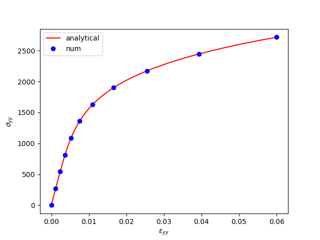
Simple Tension Test
To test the above implementation we compare our numerical results to the analytical solution for a (simple) tension test in 2D.
class AnalyticalSolution:
    """base class for ramberg osgood material solutions"""

    def __init__(self, max_load, **kwargs):
        self.load = max_load
        self.E = kwargs.get("E", 210e3)
        self.NU = kwargs.get("NU", 0.3)
        self.ALPHA = kwargs.get("ALPHA", 0.01)
        self.N = kwargs.get("N", 5.0)
        self.K = self.E / (1.0 - 2.0 * self.NU)
        self.G = self.E / 2.0 / (1.0 + self.NU)
        self.SIGY = kwargs.get("SIGY", 500.0)

    def energy(self):
        assert np.sum(self.sigma) > 0.0
        return np.trapz(self.sigma, self.eps)


class SimpleTensionSolution2D(AnalyticalSolution):
    """analytical solution for simple tension in 2D"""

    def __init__(self, max_load, **kwargs):
        super().__init__(max_load, **kwargs)

    def solve(self):
        from scipy.optimize import newton
        from sympy import symbols, Derivative, lambdify, sqrt

        E = self.E
        K = self.K
        G = self.G
        ALPHA = self.ALPHA
        SIGY = self.SIGY
        N = self.N

        def f(x, s):
            """equation to solve is eps33(x, s) = 0
            x:      sigma33
            s:      sigma22 (given as tension direction)
            """
            return (x + s) / 3.0 / K + (
                1.0 / 2.0 / G
                + 3.0
                * ALPHA
                / 2.0
                / E
                * (np.sqrt((s - x) ** 2 + x * s) / SIGY) ** (N - 1.0)
            ) * (2.0 * x - s) / 3.0

        x, s = symbols("x s")
        f_sym = (x + s) / 3.0 / K + (
            1.0 / 2.0 / G
            + 3.0 * ALPHA / 2.0 / E * (sqrt((s - x) ** 2 + x * s) / SIGY) ** (N - 1.0)
        ) * (2.0 * x - s) / 3.0
        Df = Derivative(f_sym, x)
        df = lambdify((x, s), Df.doit(), "numpy")

        s = np.linspace(0, self.load)  # sigma22
        x = np.zeros_like(s)  # initial guess
        s33 = newton(f, x, fprime=df, args=(s,), tol=1e-12)

        e11 = (s + s33) / 3.0 / K + (
            1.0 / 2.0 / G
            + 3.0
            * ALPHA
            / 2.0
            / E
            * (np.sqrt((s - s33) ** 2 + s * s33) / SIGY) ** (N - 1.0)
        ) * (-(s33 + s)) / 3.0
        e22 = (s + s33) / 3.0 / K + (
            1.0 / 2.0 / G
            + 3.0
            * ALPHA
            / 2.0
            / E
            * (np.sqrt((s - s33) ** 2 + s * s33) / SIGY) ** (N - 1.0)
        ) * (2.0 * s - s33) / 3.0
        self.sigma = s
        self.eps = e22
        return e11, e22, s
Next we define little helper functions to define neumann and dirichlet type boundary conditions.
def get_neumann(dim, force):
    f = Expression(("0.0", "F * time"), degree=0, F=force, time=0.0, name="f")

    class Top(SubDomain):
        tol = 1e-6

        def inside(self, x, on_boundary):
            return on_boundary and near(x[1], 1.0, self.tol)

    neumann = Top()
    return f, neumann


def get_dirichlet(dim, V):
    bcs = []

    class Bottom(SubDomain):
        tol = 1e-6

        def inside(self, x, on_boundary):
            return on_boundary and near(x[1], 0.0, self.tol)

    origin = CompiledSubDomain("near(x[0], 0.0) && near(x[1], 0.0)")
    bcs.append(DirichletBC(V.sub(1), Constant(0.0), Bottom()))
    bcs.append(DirichletBC(V, Constant((0.0, 0.0)), origin, method="pointwise"))
    return bcs
The function to run the simple tension test.
def simple_tension(mesh, matparam, pltshow=False):
    """
    simple tension test
    """
    ro = RambergOsgoodProblem(mesh, deg_d=1, deg_q=1, matparam)

    facets = MeshFunction("size_t", mesh, mesh.topology().dim() - 1)
    ds = Measure("ds")(subdomain_data=facets)
    facets.set_all(0)

    # external load
    max_load = 2718.0
    gdim = mesh.geometric_dimension()
    traction, neumann = get_neumann(gdim, max_load)
    neumann.mark(facets, 99)
    d_ = TestFunction(ro.V)
    force = dot(traction, d_) * ds(99)
    ro.R -= force

    # dirichlet bcs
    bcs = get_dirichlet(gdim, ro.V)
    ro.set_bcs(bcs)

    solver = NewtonSolver()
    solver.parameters["linear_solver"] = "mumps"
    solver.parameters["maximum_iterations"] = 10
    solver.parameters["error_on_nonconvergence"] = False

    x_at_top = (0.5, 1.0)

    nTime = 10
    load_steps = np.linspace(0, 1, num=nTime + 1)[1:]
    iterations = np.array([], dtype=np.int)
    displacement = [0.0, ]
    load = [0.0, ]

    for (inc, time) in enumerate(load_steps):
        print("Load Increment:", inc)
        traction.time = time
        niter, converged = solver.solve(ro, ro.d.vector())
        assert converged
        iterations = np.append(iterations, niter)

        # load displacement data
        displacement.append(ro.d(x_at_top)[1])
        load.append(traction(x_at_top)[1])

    # ### analytical solution
    displacement = np.array(displacement)
    load = np.array(load)
    sol = SimpleTensionSolution2D(max_load, **matparam)
    e11, e22, s22 = sol.solve()
    w = sol.energy()
    I = np.trapz(load, displacement)
    assert np.isclose((w - I) / w, 0.0, atol=1e-2)

    if pltshow:
        fig, ax = plt.subplots()
        ax.plot(e22, s22, "r-", label="analytical")
        ax.plot(displacement, load, "bo", label="num")
        ax.set_xlabel(r":math:`\varepsilon_{yy}`")
        ax.set_ylabel(r":math:`\sigma_{yy}`")
        ax.legend()
        ax.xaxis.set_major_formatter(FormatStrFormatter("%.2f"))
        plt.show()


if __name__ == "__main__":
    mesh = UnitSquareMesh(32, 32)
    material = {
        "E": 210e3,
        "NU": 0.3,
        "ALPHA": 0.01,
        "N": 5,
        "SIGY": 500.0
    }
    simple_tension(mesh, material, pltshow=False)
Setting pltshow=True you should see something like this: