Implicit gradient-enhanced damage model
Introduction and governing equations
A local isotropic damage model…
… is basically the modified linear-elastic momentum balance equation with
elasticity tensor \(\boldsymbol C\) - build from \(E, \nu\) or Lamé constants \(\lambda, \mu\)
damage \(\omega \in [0,1)\) that is driven by the history variable \(\kappa\)
strains \(\boldsymbol \varepsilon = \frac{1}{2}(\nabla \boldsymbol d + (\nabla \boldsymbol d)^T)\), here in Voigt notation, meaning a vector of \([\boldsymbol \varepsilon_{xx}, \boldsymbol \varepsilon_{yy}, \frac{1}{2}\boldsymbol \varepsilon_{xy}]^T\)
the KKT conditions for \(\kappa\) translate to \(\kappa = \max(\kappa, \|\boldsymbol \varepsilon\|)\), where the latter term is a scalar norm of the local strains
This local model exhibits various numerical problems, e.g. localization in single bands of elements with a vanishing fracture energy upon mesh refinement. One way to overcome these issues is to use nonlocal models that introduce a mesh-independent length scale. Here, this is by replacing the local strain norm with the nonlocal equivalent strains \(\bar \varepsilon\) as an additional degree of freedom (DOF) that is calculated by a screened Poisson equation that limits its curvature. Now, the full model reads
and details can be found, e.g., in
the original paper Gradient enhanced damage for quasi‐brittle materials, Peerlings et al., 1996 and
a more recent paper discussing alternative solution strategies Implicit–explicit integration of gradient-enhanced damage models, Titscher et al., 2019
Next, we will discuss the building blocks of the constitutive model with the code.
Remark: The functions in this section are written to work on multiple values simultaneously. So instead of evaluating a function once per scalar, we group the scalars in a (possibly huge) vector and apply the function once. This may explain some strange syntax and slicing in the code below.
Gradient damage constitutive law
import numpy as np
import ufl
from dataclasses import dataclass
Damage law
The simplest case that is used in Peerlings et al. for an analytic solution is the perfect damage model that, if inserted in the stress-strain relationship, looks like
   stress
ft |   _______________
   |  /
   | /:
   |/ :
   0--:--------------> strain
      k0
def damage_perfect(mat, kappa):
    k0 = mat.ft / mat.E
    return 1.0 - k0 / kappa, k0 / kappa ** 2
For the characteristic strain softening, an exponential damage law is commonly used. After reaching the peak load - the tensile strength \(f_t\), the curve shows an exponential drop to the residual stress \((1-\alpha)f_t\).
   stress
ft |
   |  /\
   | /: ` .
   |/ :     ` .. _____ (1-alpha)*ft
   0--:--------------> strain
      k0
def damage_exponential(mat, k):
    k0 = mat.ft / mat.E
    a = mat.alpha
    b = mat.beta

    w = 1.0 - k0 / k * (1.0 - a + a * np.exp(b * (k0 - k)))
    dw = k0 / k * ((1.0 / k + b) * a * np.exp(b * (k0 - k)) + (1.0 - a) / k)

    return w, dw
Constitutive law
Basically Hooke’s law in plane strain with the factor \((1-\omega)\).
def hooke(mat, eps, kappa, dkappa_de):
    """
    mat:
        material parameters
    eps:
        vector of Nx3 where each of the N rows is a 2D strain in Voigt notation
    kappa:
        current value of the history variable kappa
    dkappa_de:
        derivative of kappa w.r.t the nonlocal equivalent strains e
    """
    E, nu = mat.E, mat.nu
    l = E * nu / (1 + nu) / (1 - 2 * nu)
    m = E / (2.0 * (1 + nu))
    C = np.array([[2 * m + l, l, 0], [l, 2 * m + l, 0], [0, 0, m]])

    w, dw = mat.dmg(mat, kappa)

    sigma = eps @ C * (1 - w)[:, None]
    dsigma_deps = np.tile(C.flatten(), (len(kappa), 1)) * (1 - w)[:, None]

    dsigma_de = -eps @ C * dw[:, None] * dkappa_de[:, None]

    return sigma, dsigma_deps, dsigma_de
Strain norm
The local equivalent strain \(\| \boldsymbol \varepsilon \|\) is defined as
\(I_1\) is the first strain invariant and \(J_2\) is the second deviatoric strain invariant. The parameter \(k=f_c/f_t\) controls different material responses in compression (compressive strength \(f_c\)) and tension (tensile strength \(f_t\)).
See: Comparison of nonlocal approaches in continuum damage mechanics, de Vree et al., 1995
Note that the implementation here is only valid for 2D plane strain!
def modified_mises_strain_norm(mat, eps):
    nu, k = mat.nu, mat.k

    K1 = (k - 1.0) / (2.0 * k * (1.0 - 2.0 * nu))
    K2 = 3.0 / (k * (1.0 + nu) ** 2)

    exx, eyy, exy = eps[0::3], eps[1::3], eps[2::3]
    I1 = exx + eyy
    J2 = 1.0 / 6.0 * ((exx - eyy) ** 2 + exx ** 2 + eyy ** 2) + (0.5 * exy) ** 2

    A = np.sqrt(K1 ** 2 * I1 ** 2 + K2 * J2) + 1.0e-14
    eeq = K1 * I1 + A

    dJ2dexx = 1.0 / 3.0 * (2 * exx - eyy)
    dJ2deyy = 1.0 / 3.0 * (2 * eyy - exx)
    dJ2dexy = 0.5 * exy

    deeq = np.empty_like(eps)
    deeq[0::3] = K1 + 1.0 / (2 * A) * (2 * K1 * K1 * I1 + K2 * dJ2dexx)
    deeq[1::3] = K1 + 1.0 / (2 * A) * (2 * K1 * K1 * I1 + K2 * dJ2deyy)
    deeq[2::3] = 1.0 / (2 * A) * (K2 * dJ2dexy)
    return eeq, deeq
Complete constitutive class
contains the material parameters
stores the values of all integration points
calculates those fields for given \(\boldsymbol \varepsilon, \bar \varepsilon\)
@dataclass
class GDMPlaneStrain:
    # Young's modulus          [N/mm²]
    E: float = 20000.0
    # Poisson's ratio            [-]
    nu: float = 0.2
    # nonlocal length parameter [mm]
    l: float = 200 ** 0.5
    # tensile strength          [N/mm²]
    ft: float = 2.0
    # compressive-tensile ratio   [-]
    k: float = 10.0
    # residual strength factor   [-]
    alpha: float = 0.99
    # fracture energy parameters [-]
    beta: float = 100.0
    # history variable           [-]
    kappa: None = None
    # damage law
    dmg: None = damage_exponential

    def eps(self, v):
        e = ufl.sym(ufl.grad(v))
        return ufl.as_vector([e[0, 0], e[1, 1], 2 * e[0, 1]])

    def kappa_kkt(self, e):
        if self.kappa is None:
            self.kappa = self.ft / self.E
        return np.maximum(e, self.kappa)

    def evaluate(self, eps_flat, e):
        kappa = self.kappa_kkt(e)
        dkappa_de = (e >= kappa).astype(int)

        eps = eps_flat.reshape(-1, 3)
        self.sigma, self.dsigma_deps, self.dsigma_de = hooke(
            self, eps, kappa, dkappa_de
        )
        self.eeq, self.deeq = modified_mises_strain_norm(self, eps_flat)

    def update(self, e):
        self.kappa = self.kappa_kkt(e)
from gdm_constitutive import *
from helper import *
from dolfin.cpp.log import log
Quadrature space formulation
- Degrees of freedom in a mixed function space
u = [d, e]
u = total mixed vector
d = displacement field \(\boldsymbol d\)
e = nonlocal equivalent strain field \(\bar \varepsilon\)
Momentum balance + Screened Poisson …
Rd = eps(dd) : sigma(eps(d), e) * dx
Re = de * e * dx + grad(de) . l ** 2 * grad(e) * dx  - de * eeq(eps) * dx
plus their derivatives
dRd/dd = eps(dd) : (dSigma_deps) * eps(d)) * dx
dRd/de = de * (dSigma_de * eps(d)) *dx
dRe/dd = eps(dd) * (-deeq_deps) * e * dx
dRe/de = de * e * dx + grad(de) . l**2 * grad(e) * dx
The trivial terms in the equations above are implemented using FEniCS
forms. The non-trivial ones are defined as functions with prefix q_ in
appropriately-sized quadrature function spaces. The values for those functions
are calculated in the GDMPlaneStrain class above.
class GDM(NonlinearProblem):
    def __init__(self, mesh, mat, **kwargs):
        NonlinearProblem.__init__(self)
        self.mat = mat
        deg_d = 2
        deg_e = 2
        deg_q = 2

        metadata = {"quadrature_degree": deg_q, "quadrature_scheme": "default"}
        dxm = dx(metadata=metadata)

        cell = mesh.ufl_cell()

        # solution field
        Ed = VectorElement("CG", cell, degree=deg_d)
        Ee = FiniteElement("CG", cell, degree=deg_e)

        self.Vu = FunctionSpace(mesh, Ed * Ee)
        self.Vd, self.Ve = self.Vu.split()
        self.u = Function(self.Vu, name="d-e mixed space")

        # generic quadrature function spaces
        q = "Quadrature"
        voigt = 3
        QF = FiniteElement(q, cell, deg_q, quad_scheme="default")
        QV = VectorElement(q, cell, deg_q, quad_scheme="default", dim=voigt)
        QT = TensorElement(q, cell, deg_q, quad_scheme="default", shape=(voigt, voigt))
        VQF, VQV, VQT = [FunctionSpace(mesh, Q) for Q in [QF, QV, QT]]

        # quadrature function
        self.q_sigma = Function(VQV, name="current stresses")
        self.q_eps = Function(VQV, name="current strains")
        self.q_e = Function(VQF, name="current nonlocal equivalent strains")
        self.q_k = Function(VQF, name="current history variable kappa")
        self.q_eeq = Function(VQF, name="current (local) equivalent strain (norm)")

        self.q_dsigma_deps = Function(VQT, name="stress-strain tangent")
        self.q_dsigma_de = Function(VQV, name="stress-nonlocal-strain tangent")
        self.q_deeq_deps = Function(VQV, name="equivalent-strain-strain tangent")

        dd, de = TrialFunctions(self.Vu)
        d_, e_ = TestFunctions(self.Vu)
        d, e = split(self.u)

        try:
            f_d = kwargs["f_d"]
        except:
            f_d = Constant(1.0)

        eps = self.mat.eps
        self.R = f_d * inner(eps(d_), self.q_sigma) * dxm
        self.R += e_ * (e - self.q_eeq) * dxm
        self.R += dot(grad(e_), mat.l ** 2 * grad(e)) * dxm

        self.dR = f_d * inner(eps(d_), self.q_dsigma_deps * eps(dd)) * dxm
        self.dR += f_d * inner(eps(d_),  self.q_dsigma_de * de) * dxm
        self.dR += e_ * (de - dot(self.q_deeq_deps, eps(dd))) * dxm
        #∂grad(e)/∂e de = linear terms of grad(e+de) = grad(de)
        self.dR += dot(grad(e_), mat.l ** 2 * (grad(de))) * dxm

        self.calculate_eps = LocalProjector(eps(d), VQV, dxm)
        self.calculate_e = LocalProjector(e, VQF, dxm)

        self.assembler = None

    def evaluate_material(self):
        # project the strain and the nonlocal equivalent strains onto
        # their quadrature spaces and ...
        self.calculate_eps(self.q_eps)
        self.calculate_e(self.q_e)

        eps_flat = self.q_eps.vector().get_local()
        e = self.q_e.vector().get_local()

        # ... "manually" evaluate_material the material ...
        self.mat.evaluate(eps_flat, e)

        # ... and write the calculated values into their quadrature spaces.
        set_q(self.q_eeq, self.mat.eeq)
        set_q(self.q_deeq_deps, self.mat.deeq)
        set_q(self.q_sigma, self.mat.sigma)
        set_q(self.q_dsigma_deps, self.mat.dsigma_deps)
        set_q(self.q_dsigma_de, self.mat.dsigma_de)

    def update(self):
        self.calculate_e(self.q_e)
        self.mat.update(self.q_e.vector().get_local())
        set_q(self.q_k, self.mat.kappa) # just for post processing

    def set_bcs(self, bcs):
        # Only now (with the bcs) can we initialize the assembler
        self.assembler = SystemAssembler(self.dR, self.R, bcs)

    def F(self, b, x):
        if not self.assembler:
            raise RuntimeError("You need to `.set_bcs(bcs)` before the solve!")
        self.evaluate_material()
        self.assembler.assemble(b, x)

    def J(self, A, x):
        self.assembler.assemble(A)
- Remark: Subclassing from
dolfin.NonlinearProblem… … is rather straight forward as we only need to pass our forms and boundary conditions to the
dolfin.SystemAssemblerand call it in the overwritten methodsF(assembles the out-of-balance forces) andJ(assembles the tangent) …… and allows us to directly use
dolfin.NewtonSolver- the Newton-Raphson implementation of FEniCS. Note that this algorithm (as probably every NR) always evaluatesFbeforeJ. So it is sufficient to perform theGDM.evaluate_materialonly inF.
Examples
Comparison with the analytic solution
The Peerlings paper cited above includes a discussion on an analytic solution
of the model for the damage_perfect damage law. A 1D bar of length \(L\)
(here modeled as a thin 2D structure) has a cross section reduction \(\alpha\)
over the length of \(W\) and is loaded by a displacement BC \(\Delta L\).
- Three regions form:
damage in the weakened cross section
damage in the unweakened cross section
no damage
and the authors provide a solution of the PDE system for each of the regions.
Finding the remaining integration constants is left to the reader. Here, it
is solved using sympy. We also subclass from dolfin.UserExpression to
interpolate the analytic solution into function spaces or calculate error norms.
import numpy as np


class PeerlingsAnalytic:
    def __init__(self):
        self.L, self.W, self.deltaL, self.alpha = 100.0, 10.0, 0.05, 0.1
        self.E, self.kappa0, self.l = 20000.0, 1.0e-4, 1.0

        self._calculate_coeffs()

    def _calculate_coeffs(self):
        """
        The analytic solution is following Peerlings paper (1996) but with
        b(paper) = b^2 (here)
        g(paper) = g^2 (here)
        c(paper) = l^2 (here)
        This modification eliminates all the sqrts in the formulations.
        Plus: the formulation of the GDM in terms of l ( = sqrt(c) ) is
        more common in modern publications.
        """

        # imports only used here...
        from sympy import Symbol, symbols, N, integrate, cos, exp, lambdify
        import scipy.optimize

        # unknowns
        x = Symbol("x")
        unknowns = symbols("A1, A2, B1, B2, C, b, g, w")
        A1, A2, B1, B2, C, b, g, w = unknowns

        l = self.l
        kappa0 = self.kappa0

        # 0 <= x <= W/2
        e1 = C * cos(g / l * x)
        # W/2 <  x <= w/2
        e2 = B1 * exp(b / l * x) + B2 * exp(-b / l * x)
        # w/2 <  x <= L/2
        e3 = A1 * exp(x / l) + A2 * exp(-x / l) + (1 - b * b) * kappa0

        de1, de2, de3 = e1.diff(x), e2.diff(x), e3.diff(x)

        eq1 = N(e1.subs(x, self.W / 2) - e2.subs(x, self.W / 2))
        eq2 = N(de1.subs(x, self.W / 2) - de2.subs(x, self.W / 2))
        eq3 = N(e2.subs(x, w / 2) - kappa0)
        eq4 = N(de2.subs(x, w / 2) - de3.subs(x, w / 2))
        eq5 = N(e3.subs(x, w / 2) - kappa0)
        eq6 = N(de3.subs(x, self.L / 2))
        eq7 = N((1 - self.alpha) * (1 + g * g) - (1 - b * b))
        eq8 = N(
            integrate(e1, (x, 0, self.W / 2))
            + integrate(e2, (x, self.W / 2, w / 2))
            + integrate(e3, (x, w / 2, self.L / 2))
            - self.deltaL / 2
        )

        eqs = [
            lambdify(unknowns, eq) for eq in [eq1, eq2, eq3, eq4, eq5, eq6, eq7, eq8]
        ]

        def global_func(x):
            return np.array([eqs[i](*x) for i in range(8)])

        result = scipy.optimize.root(
            global_func, [0.0, 5e2, 3e-7, 7e-3, 3e-3, 3e-1, 2e-1, 4e1]
        )
        if not result["success"]:
            raise RuntimeError(
                "Could not find the correct coefficients. Try to tweak the initial values."
            )

        self.coeffs = result["x"]

    def e(self, x):
        A1, A2, B1, B2, C, b, g, w = self.coeffs
        if x <= self.W / 2.0:
            return C * np.cos(g / self.l * x)
        elif x <= w / 2.0:
            return B1 * np.exp(b / self.l * x) + B2 * np.exp(-b / self.l * x)
        else:
            return (
                (1.0 - b * b) * self.kappa0
                + A1 * np.exp(x / self.l)
                + A2 * np.exp(-x / self.l)
            )
from gdm_analytic import PeerlingsAnalytic

class PeerlingsAnalyticExpr(UserExpression, PeerlingsAnalytic):
    def __init__(self, **kwargs):
        PeerlingsAnalytic.__init__(self)
        UserExpression.__init__(self, **kwargs)

    def eval(self, value, x):
        value[0] = self.e(x[0])
Using this, we can rebuild the example with our GDM nonlinear problem and
compare.
def gdm_error(n_elements):
    """
    ... evaluated in 2D
    """
    e = PeerlingsAnalyticExpr(degree=4)

    mesh = RectangleMesh(Point(0.0, 0.0), Point(e.L / 2.0, 1), n_elements, 1)
    mat = GDMPlaneStrain(E=e.E, nu=0.0, ft=e.E * e.kappa0, l=e.l, dmg=damage_perfect)

    area = Expression(
        "x[0] <= W/2. ? 10.0 * (1. - a) : 10.0", W=e.W, a=e.alpha, degree=0
    )
    gdm = GDM(mesh, mat, f_d=area)

    bc_expr = Expression("t*d", degree=0, t=0, d=e.deltaL / 2)
    bc0 = DirichletBC(gdm.Vd, (0.0, 0.0), plane_at(0.0))
    bc1 = DirichletBC(gdm.Vd.sub(0), bc_expr, plane_at(e.L / 2.0))
    gdm.set_bcs([bc0, bc1])

    solver = NewtonSolver()
    solver.parameters["linear_solver"] = "mumps"
    solver.parameters["maximum_iterations"] = 10
    solver.parameters["error_on_nonconvergence"] = False

    for t in np.linspace(0.0, 1.0, 11):
        bc_expr.t = t
        assert solver.solve(gdm, gdm.u.vector())[1]

    e_fem = gdm.u.split()[1]
    return errornorm(e, e_fem)
This error should converge to zero upon mesh refinement and can be used to determine the order of convergence of the model.
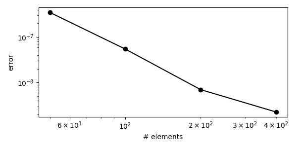
def convergence_test():
    ns = [50, 100, 200, 400]
    errors = []
    for n in ns:
        errors.append(gdm_error(n))

    ps = []
    for i in range(len(ns) - 1):
        p = np.log(errors[i] - errors[i + 1]) / np.log(1.0 / ns[i] - 1.0 / ns[i + 1])
        ps.append(p)

    import matplotlib.pyplot as plt
    plt.figure(figsize=(6, 3))
    plt.loglog(ns, errors, "-ko")
    plt.xlabel("# elements")
    plt.ylabel("error")
    plt.tight_layout()
    plt.savefig("gdm_convergence.png")
    plt.show()
    print(ps)
Three-point bending test
Just a more exciting example.
Note that we pass our GDM class as well as the linear solver as a parameter.
These can be modified to use an iterative solver.
def three_point_bending(problem=GDM, linear_solver=LUSolver("mumps")):
    LX = 2000
    LY = 300
    LX_load = 100

    mesh = RectangleMesh(Point(0, 0), Point(LX, LY), 100, 15)
    mat = GDMPlaneStrain()
    gdm = problem(mesh, mat)

    bcs = []
    left = point_at((0.0, 0.0), eps=0.1)
    right = point_at((LX, 0.0), eps=0.1)
    top = within_range([(LX - LX_load) / 2.0, LY], [(LX + LX_load) / 2, LY], eps=0.1)

    bc_expr = Expression("d*t", degree=0, t=0, d=-3)
    bcs.append(DirichletBC(gdm.Vd.sub(1), bc_expr, top))
    bcs.append(DirichletBC(gdm.Vd.sub(0), 0.0, left, method="pointwise"))
    bcs.append(DirichletBC(gdm.Vd.sub(1), 0.0, left, method="pointwise"))
    bcs.append(DirichletBC(gdm.Vd.sub(1), 0.0, right, method="pointwise"))

    gdm.set_bcs(bcs)

    solver = NewtonSolver(MPI.comm_world, linear_solver, PETScFactory.instance())
    solver.parameters["linear_solver"] = "mumps"
    solver.parameters["maximum_iterations"] = 10
    solver.parameters["error_on_nonconvergence"] = False

    def solve(t, dt):
        bc_expr.t = t
        return solver.solve(gdm, gdm.u.vector())

    ld = LoadDisplacementCurve(bcs[0])
    ld.show()
    if not ld.is_root:
        set_log_level(LogLevel.ERROR)

    fff = XDMFFile("output.xdmf")
    fff.parameters["functions_share_mesh"] = True
    fff.parameters["flush_output"] = True
    plot_space = FunctionSpace(mesh, "DG", 0)

    def pp(t):
        gdm.update()

        # this fixes XDMF time stamps
        import locale
        locale.setlocale(locale.LC_NUMERIC, "en_US.UTF-8")
        fff.write(gdm.u.split()[0], t)
        fff.write(gdm.u.split()[1], t)

        # plot the damage
        q_k = gdm.q_k
        q_w = Function(q_k.function_space())
        set_q(q_w, mat.dmg(mat, q_k.vector().get_local())[0])
        w = project(q_w, plot_space)
        w.rename("w", "w")
        fff.write(w, t)

        ld(t, assemble(gdm.R))

    TimeStepper(solve, pp, gdm.u).adaptive(1.0, dt=0.1)


if __name__ == "__main__":
    assert gdm_error(200) < 1.0e-8
    convergence_test()
    three_point_bending()
    # list_timings(TimingClear.keep, [TimingType.wall])
Extensions
make everything dimension independent