Force spectroscopy data#
Introduction#
Force spectroscopy data is usually acquired experimentally by atomic force microscopy (AFM) and has its challenges when an automated analysis of the data is attempted, f. e. with SOFA (SOftware for Force Analysis). For one it is unique to this spectroscopic data, that the shift of the abscissa is not inherently known from the measurement. An additional challenge is, that the spectrum is not monotonous. The change of regimes of attractive and repulsive forces results in a singularity, called the jump to contact (JTC). Data in the attractive respectively repulsive regime can be described by general theories, such as van der Waals attraction and Hertz contact, but one single expression which describes the full spectroscopic range does not exist.
With SOFA we develop a software aiming for a robust algorithm, which will be able to handle all varieties of force spectroscopy data. In order to test this capability, reliable synthetic test data is required for which SyFoS was written. SyFoS mirrors the experimental acquisition of data and successively builds force spectroscopy data, taking material parameter and experimental parameter into account. All parameters can be specified by the user via a graphical user interface. To achieve realistic challenges in the test data sets a noise level and data offsets are added. The software is stored in GitHub.
Creating synthetic force spectroscopy data#
Under the umbrella term of force spectroscopy usually force curves, such as force distance curves (FDC) are understood. The process of generating an ideal curve is explained in Creation of ideal force curves. In Creating force curves with artefacts the most common sources of deviation of real force curves from an ideal force curve are shown, which can be added to the ideal curve in SyFoS. Since it is very common in an experiment to record more than one force curve, for example in a series or in an array (also called force volume) this option is also given in SyFoS (Creating force curve arrays).
Creation of ideal force curves#
SyFoS is designed to mirror force spectroscopy measurements, more precisely the acquisition of force-distance curves (FDC). Below the FDC experiment is described.
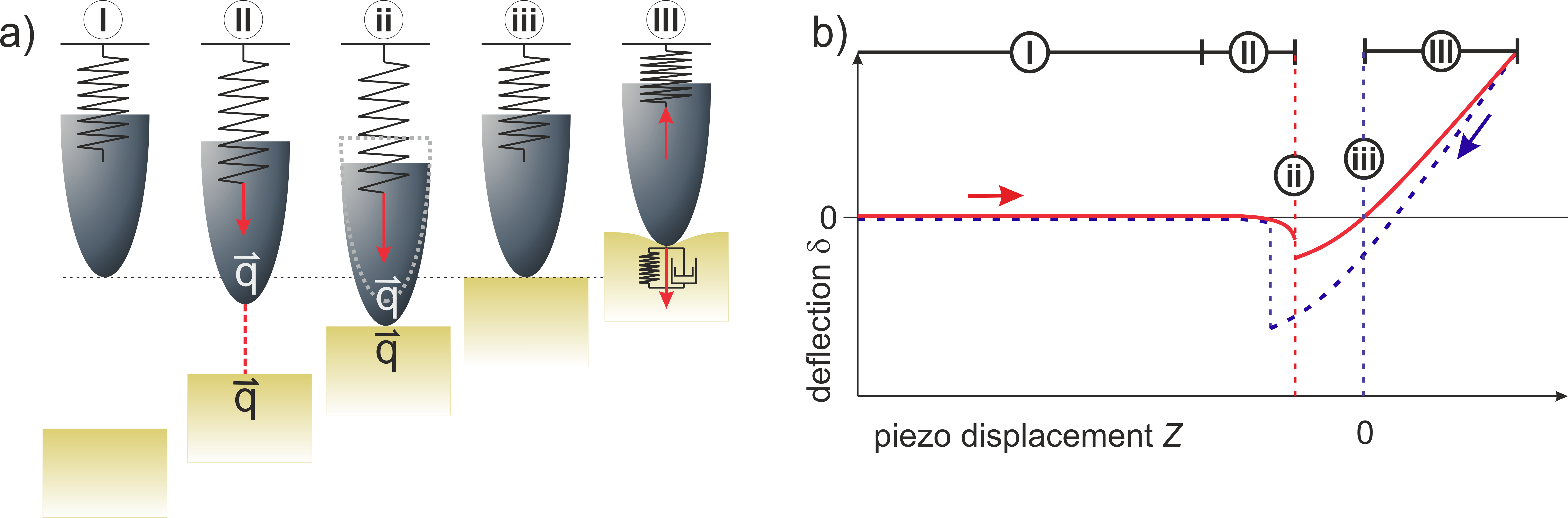
Figure 1: a) representation of tip-sample interactions b) schematic drawing of a FDC with (I) zero-line, (II) regime of attractive forces, (ii) JTC, (iii) contact and (III) contact line.#
During the acquisition of a FDC the AFM probe, a paraboloid shaped tip with radius \(R\) is hold at a fixed x,y position while it approaches the sample surface by use of a Z-piezo. The tip is attached at a cantilever which can be described as an elastic spring following Hooke’s law:
with force \(F\), spring constant \(k_c\) of the cantilever and cantilever deflection \(δ\). In this way the forces acting on the tip are measured by recording the deflection \(δ\) of the cantilever. While decreasing the distance between tip and sample, the cantilever deflects toward the sample (attractive forces) or away (repulsive forces), depending on which interacting forces are dominant.
Due to the sum of all interacting forces, a FDC shows three typical regimes upon approach as depicted in Figure 1.
zero line (I)
When tip and sample are far away from each other and interacting forces are not detectable, the deflection signal \(δ\) is zero which equals the free equilibrium position of the cantilever.
regime of attractive forces \(F_{attr}\) (II)
Upon further approach of sample and tip, attractive forces start to govern, and the cantilever is bend towards the sample. The attractive forces between sample and tip increase up to a point when their gradient exceeds the spring constant \(k_c\).
jump to contact (JTC) (ii)
A discontinuity where the system is not in equilibrium and the tip snaps onto the sample.
contact (iii)
Attractive and repulsive forces are in balance and the cantilever has reached its equilibrium position again.
contact line (III)
Upon further approach the repulsive forces are dominant, and the cantilever is pushed away from the sample. The deflection \(δ\) corresponds to the applied force \(F\) by Hooke’s law (1). At a maximum piezo displacement \(Z_{max}\), the approach is stopped, and the sample is withdrawn until the contact is lost at jump off contact (JOC) and the zero line is reached again (only shown in Figure 1 b, blue dashed line). In SyFoS, only the approach part of acquired curves is considered.
This experiment is mirrored in SyFoS, by assigning the according cantilever deflection \(δ_i\) to a given piezo displacement \(Z_i\) for a range of \(Z\) values starting from \(Z_0\) and increasing by \(dZ\) until \(Z_{max}\) is reached (see experimental set-up for more detailed information about the parameters). Due to the discontinuity of the JTC, SyFoS creates the synthetic data by a case-by-case analysis, starting in the zero line and attractive regime.
Zero line#
For every given piezo displacement point \(Z_i\) the actual tip-sample distance \(ζ_i\) is calculated:
For the given tip-sample distance \(ζ_i\) the van der Waals interaction \(F_{vdW,i}\) is calculated by:
with Hamaker constant \(A\), tip radius \(R\), deflection \(δ\), piezo displacement \(Z\) and tip-sample distance \(ζ\).
From the acting van der Waals force \(F_{vdW,i}\) the resulting deflection \(δ_{(i+1)}\) is determined by Hooke’s law (1). From this deflection \(δ_{(i+1)}\) and \(Z_{(i+1)}=Z_i+dZ\) the true tip-sample distance \(ζ_{(i+1)}\) is calculated and the \(F_{vdW,i+1}\) is calculated.
This continues until the condition for JTC is met, which is the case when the gradient (first derivative) of the attractive Forces (2) equals or exceeds \(k_c\):
Attractive Part#
In this case SyFoS sets the tip-sample distance to \(ζ≡0\) and assigns the according \(δ_{JTC}\) to the piezo displacement \(Z_i\) with \(δ_{JTC}<0\).
This is continued until \(Z_i\) and \(δ(Z_i)\) reach zero.
We want to point out, that in the region from JTC to contact (see Figure 1 II), a mixture of attractive and repulsive forces acts on the tip-sample system, which cannot be correctly described without taking time-dependent parameters into account. Since this part of the force curve is not subject to any subsequent use as test data, there is no attempt to implement the necessary theory on the cost of over-complicating the acquisition of synthetic force curves. For this we refer to nanohub.
Contact Part#
Until \(Z_{max}\) is reached the dominance of repulsive forces (see Figure 1 III) is assumed. Here, instead of a tip-sample distance \(ζ\) the deformation \(D\) has to be considered, which is calculated by:
with deflection \(δ\) and piezo displacement \(Z\)
In order to calculate the correct deformation \(D\) a theory of continuums mechanics has to be applied, in case of SyFoS we chose to use Hertz contact of a sphere versus a plane is used:
With applied force \(F\), tip radius \(R\) and the reduced Young’s modulus \(E_{tot}\).
with the Young’s modulus of the two materials \(E_{tip}\) and \(E_{sample}\) and their poisson ratios \(ν_{tip}\) and \(ν_{sample}\).
SyFoS is creating the deflection \(δ\) in dependence of the z piezo displacement \(δ(Z_i)\). To accommodate this in the Hertz theory (6) deformation \(D\) and force \(F\) have to by expressed through deflection \(δ\) and z piezo displacement \(Z\) by using Hooke’s law (1) and the equation for deformation (5).
With spring constant \(k_c\), tip radius \(R\) and reduced Young’s modulus \(E_{tot}\).
For solving the equation, the constant parameters \(k_c\), \(R\) and \(E_{tot}\) are substituted by \(a=\frac{k_c}{\sqrt{r}E_{tot}}\) leading to one real solution:
The imaginary solutions are not taken into consideration for SyFoS since \(Z\), \(δ\) and a have always positive values (>0).
Creating force curves with artefacts#
Experimentally acquired force curves differ in three respects from ideal force curves. First experimental curves usually experience a virtual deflection, which causes the deflection \(δ ≠ 0\) for the equilibrium position of the cantilever. This can be simply an offset or also a linear or sinusoidal function δ(Z). Second in FDC experiments the tip-sample distance is actually not known exactly. Since the topography of the sample is usually not perfectly smooth the point of JTC can be expected for a certain range of piezo displacements Z, but the exact point of contact (Z≡0) has to be established later during analysis. Thirdly, as all experimental data, also FDC suffer from noise. All three disturbance values can be added in SyFoS to the ideal curves (see artefact parameters), in order to make the synthetic force spectroscopy data more realistic.
Creating force curve arrays#
It is very common to record force distance curves in a x-y grid (mapping, also called force volume) rather than having single force-distance curves at arbitrary points. When recorded in a grid, the force spectroscopy data has an additional spatial information which is important for inhomogeneous samples. It is also useful for homogeneous samples because one acquires an array of curves which can be averaged and statistically treated for errors. To mirror this in SyFoS arrays can also be created, consisting of single curves which exhibit artefacts.